The Hunt for OTV-7

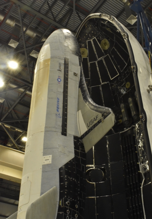
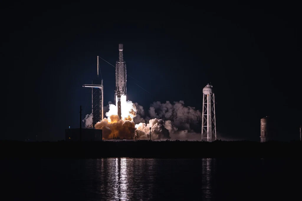
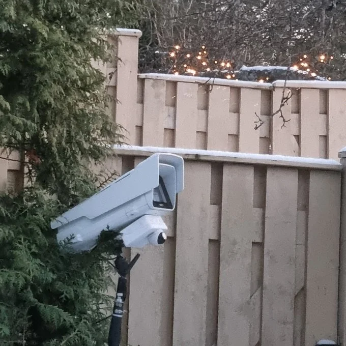
On a dark late December winter night the United States military launched its secretive X-37B spaceplane atop a Falcon 9 heavy rocket from Kennedy Space Center. After watching the rocket slip from sight and the side boosters return nothing was seen from the spaceplane until the night of February 7, 2024 when amateur satellite observer Tomi Simola found something unusual, read his story below…

Read more: The Hunt for OTV-7

Into the Dark

At 01:07 UTC December 29, 2023, the US Space Force (USSF) launched their latest X-37B spaceplane mission referred to at Orbital Test Vehicle (OTV) 7 into a highly classified secret orbit.

OTV-7 launched atop a SpaceX Falcon 9 Heavy on December 29, 2023.

Unlike earlier missions this launch was not targeting a low Earth orbit (LEO). The limited details shared to the public in Notice To Airmen (NOTAMs) revealed the spaceplane was likely targeting a high Earth orbit (HEO). Dr. Marco Langbroek conducted an analysis of the NOTAM information and shared a plausible trajectory for OTV-7.

Macro LangBroek’s analysis and suggested search trajectory for OTV-7.

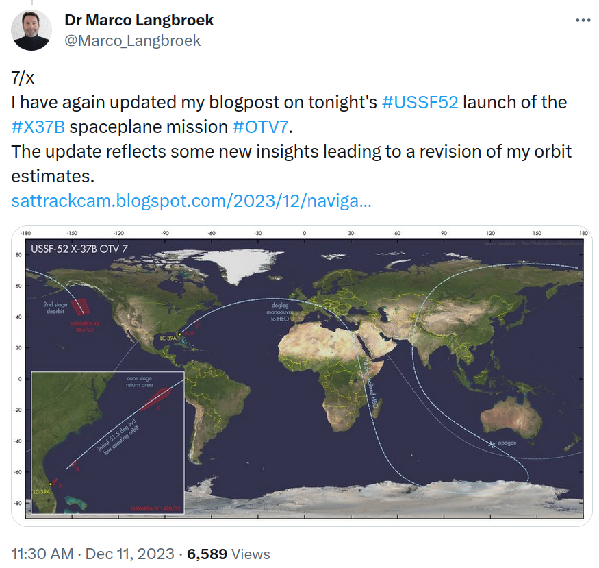
Unfortunately, the time of the launch placed most of the trajectory in Earth’s shadow hiding the spaceplane from view during most of its initial coast orbit and while climbing to apogee it would be lost in the glare of the Sun during daylight.

To make the search more challenging X-37B’s are not known to emit on traditional Tracking Telemetry and Control (TT&C) radio frequency bands and likely use the National Reconnaissance Office’s (NRO) classified Satellite Data Service (SDS) and inter-satellite communications links making it exceeding difficult to track emissions from the spaceplane. 

One thing we did have going for us to search for on radio in the dark and later in the glare of the Sun was the final stage of the Falcon 9 Heavy. Given the NOTAMs revealed the rocket stage would be de-orbited over the northern Pacific Ocean thus its mission would likely carry on to at least apogee where it would conduct a de-orbit burn to lower its perigee to below the Earth’s surface to safely de-orbit the stage in the remote ocean area noted on the NOTAM.

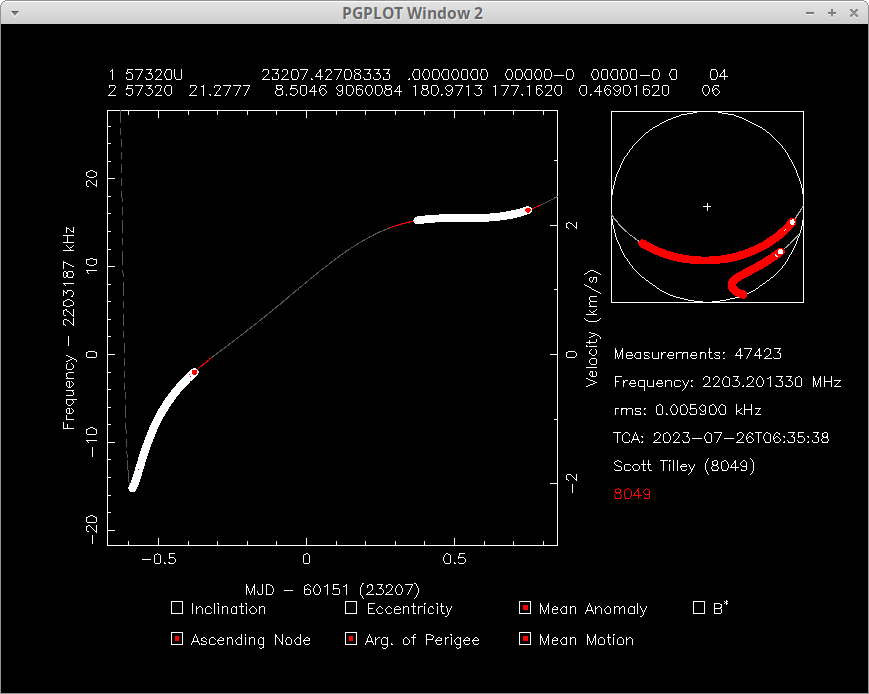
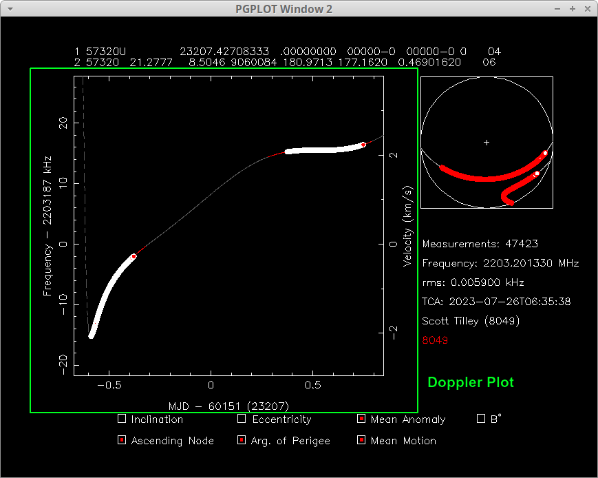
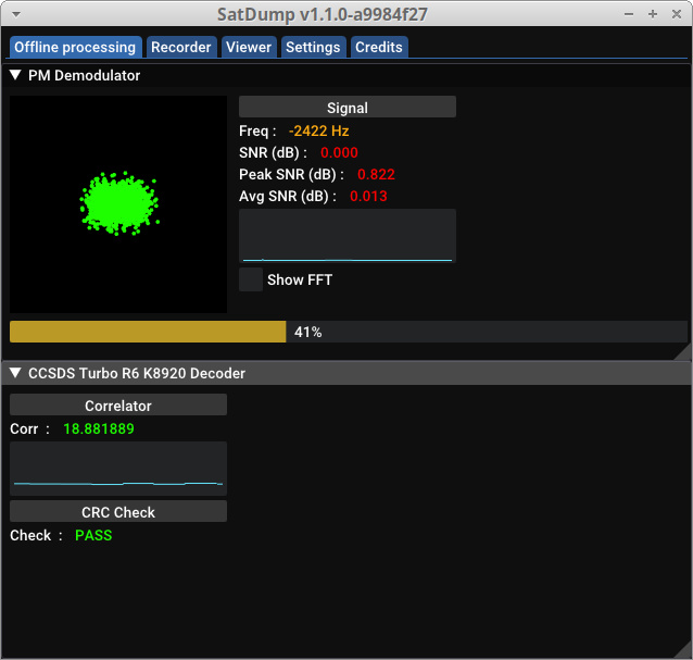
Using Federal Communications Commission (FCC) filings we found the particular paperwork for the USSF-52 launch as submitted by SpaceX and knew that the final stage rocket should be emitting on 2232.5, 2247.5, 2255.5 and/or 2272.5MHz.

A group of amateur satellite trackers in Europe and western Australia where organized in an attempt to gather radio data from the Falcon 9’s final stage in an attempt to confirm the actual trajectory of the OTV-7 through this indirect means and hopefully allow for its optical recovery later.

Using Marco LangBroek’s search TLE, a radio observer in Western Australia was right under the suspected track of the OTV-7 and its rocket stage.

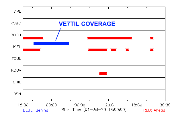
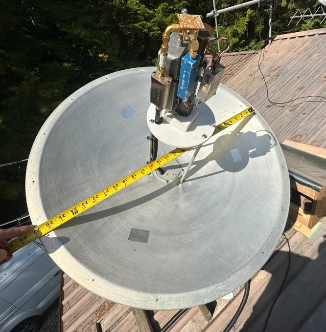
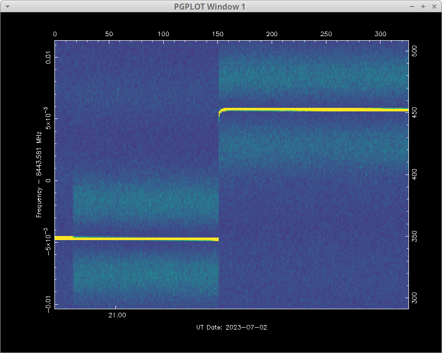
The observer in western Australia maintained vigilance for the entire expected pass of OTV-7 and its respective rocket booster. Guidance was provided to the station to conduct scans of the clear sky from 2200-2300MHz from the site using their 1m dish antenna in an effort to find the rocket booster’s emissions on S-band. We heard many signals from many other missions but nothing form OTV-7’s rocket booster. Therefore, either the rocket booster wasn’t emitting, which would be highly unlikely considering past observing experience or the trajectory guess for OTV-7 was not accurate enough to place the rocket booster in the sky above the observer in western Australia. 

To Planar Scan or Stare into Space…?

It seemed like our only chance to find OTV-7 using Marco Langbroek’s reasonable analysis of NOTAM data had resulted in failure and most likely a long search would need to be performed to find OTV-7. Two possible strategies to find OTV-7 could have been reasonably considered. One, a planar search which assumes OTV-7 was on the orbital plane Marco’s trajectory stated but it was not in the location in the plane we thought. Two, multiple observers could just stare into space and with patience OTV-7 would pass sooner or most likely later through the field of view of someone.

What is a planar search? A satellite once launched into space is in a fixed plane with respect to the stars and it will stay in that orbital plane for all practical purposes unless something adds or removes energy from the object. The effects of atmospheric drag ,solar radiation pressure, venting etc. can cause the spacecraft’s position within an orbital plane to change over time creating uncertainty of where within the orbital plane the satellite is. To recover an object in a known orbital plane one can search the plane by scanning along it for a prolonged period of time and eventually you will find your wayward satellite. However, this assumes you know the orbital plane correctly.

In our radio search for the final rocket stage which should have been very close to OTV-7, we actually compensated for this by conducting a broader search of the track and sky for some hours and would have likely found the rocket’s emissions had the orbital plane guess been close. Another factor is the timing of arriving in the orbit was fairly constrained limiting the search area along the orbit plane. This left us to conclude that OTV-7 was most likely not in the orbital plane Marco’s analysis suggested. Thus an planar search of the plane Marco suggested was likely going to be very laborious and not result in recovering OTV-7.

Marco Langbroek, Tomi Simola and Scott Tilley discuss a search strategy on X (formerly Twitter) for OTV-7.

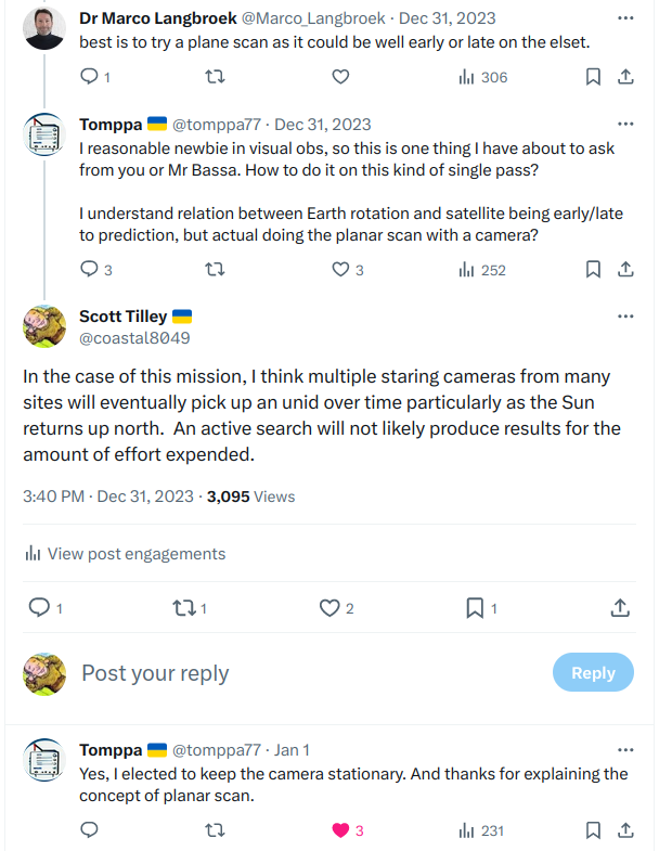
Based on what we knew, it was agreed that staring into space may be the best strategy. You may be wondering and rightfully point out that space is pretty vast and staring at a fixed small spot may never produce results. It’s counter-intuitive but the fact is a satellite is in a fixed orbit. In this case we roughly knew the orbital geometry of our target and had a pretty good idea that if we aimed a camera at an intelligently chosen fixed spot and waited long enough the satellite would pass through and we would know it was our target because almost all other objects on orbit are known and catalogued or would be in different orbits and could be excluded. 

OTV-7’s actual passes over Tomi Simola’s observing station for 30 days. Notice the patterns in the trajectory. If you know something about the inclination and shape of the orbit you can stare at optimal places in the sky to improve your chances of the spacecraft passing through your field of view.

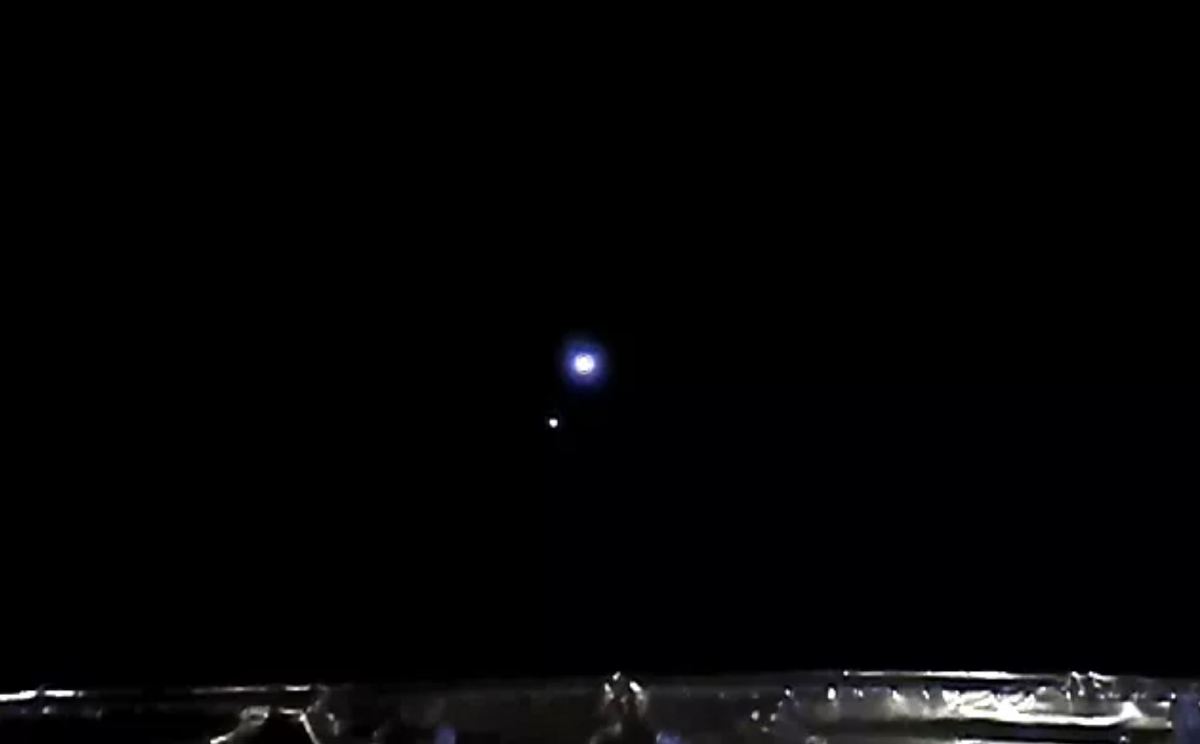
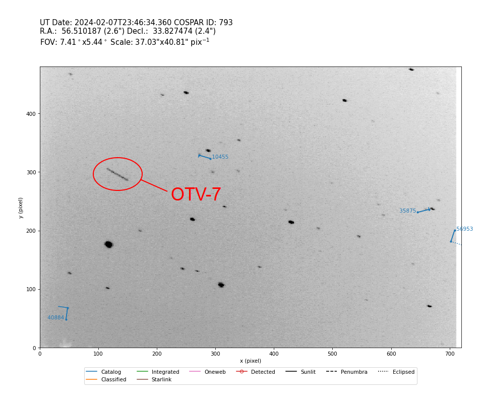
This is what Tomi Simola did to find OTV-7, he setup a light sensitive camera and connected it to a computer to record the results and excluded every object that passed through his field of view for literally weeks until an unidentified object passed through the field of view that matched OTV-7’s characteristics. 

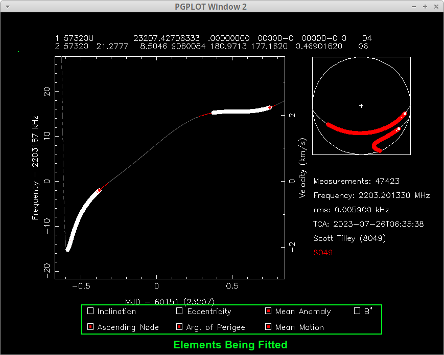
On the night of February 7, 2024, Tomi Simola recovered OTV-7 and made these observations with his staring camera. Once you have even a limited set of short arc observations you can start to generate orbital elements from the data and start to narrow down the identity of the object. After consulting Mike McCants an expert on classified objects on orbit the identity was quickly firmed up as the orbital data came in on successive nights.

Tomi Simola’s discovery image of OTV-7 from February 7, 2024.

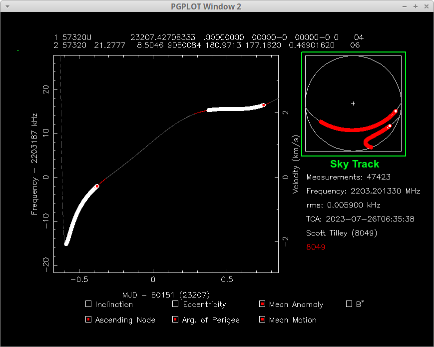
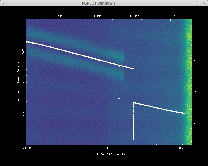
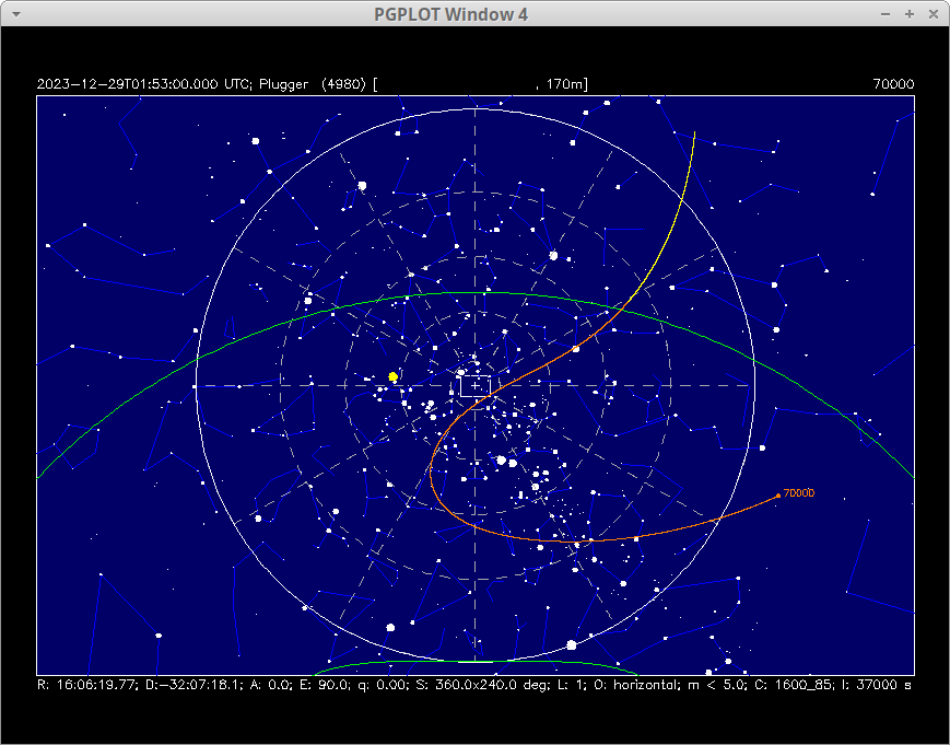
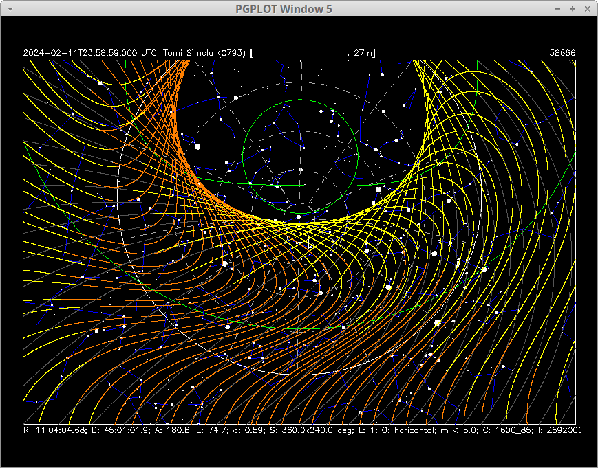
It turned out that our assumption that OTV-7 was in a different orbital plane than Marco’s reasoned guess was correct. Below you can see the dramatic difference in the sky track from the observer in western Australia for OTV-7. Much of the track was obscured by trees and other obstacles at the ground station. OTV-7 quickly passed through the ground station’s clear area of sky spent most of the pass low on the south eastern horizon obscured by trees and then as it descended from apogee passed quickly through the observable sky and disappeared…

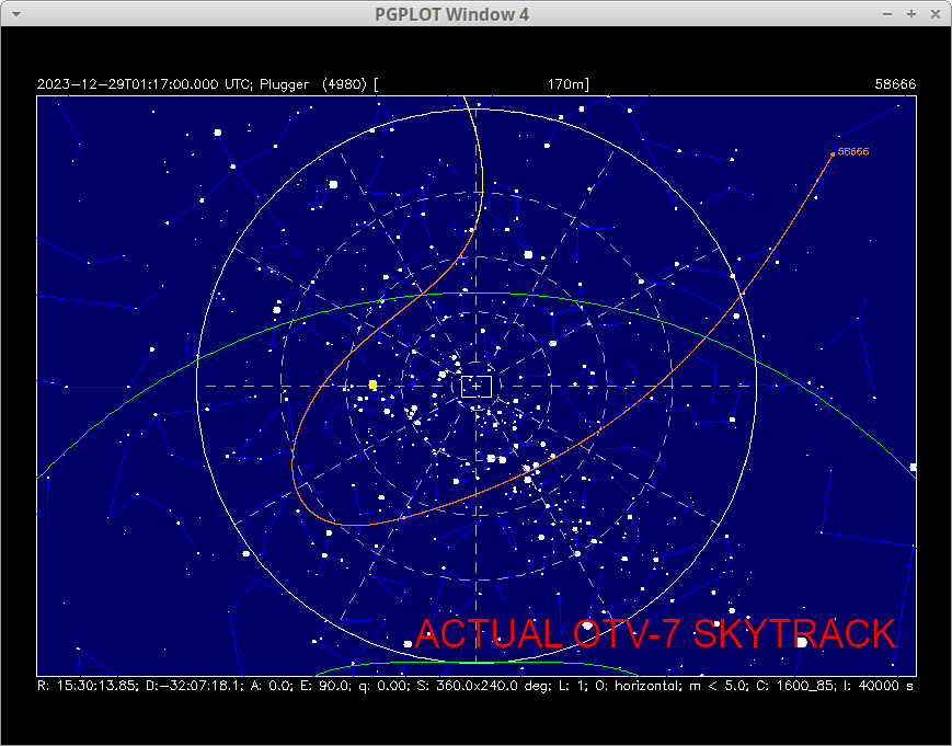
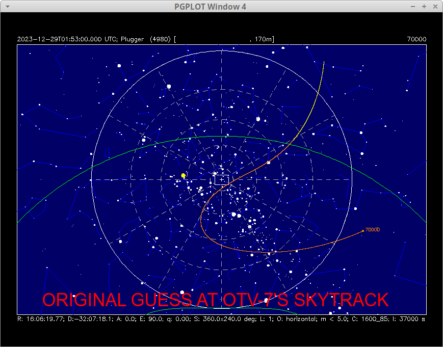
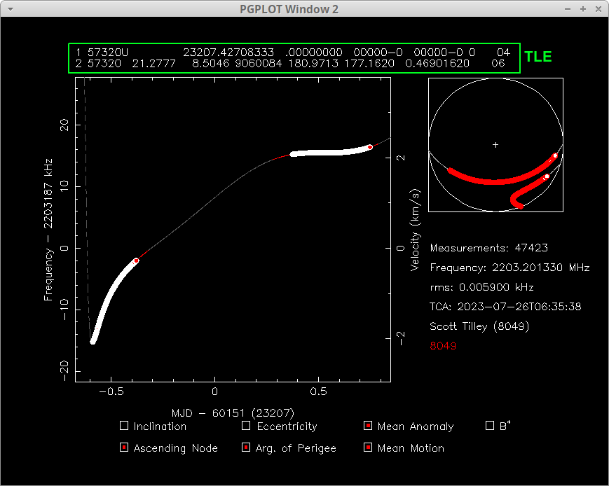
For the record here are the initial guess TLE vs. the TLE developed from Tomi Simola’s observations of OTV-7 after it was recovered.

USSF-52 OTV 7 for launch on 29 Dec 2023 01:07:00 UTC
1 70000U 23999A 23363.06545139 .00000000 00000-0 00000-0 0 02
2 70000 074.0000 341.4480 7418186 136.2072 360.0000 02.14201823 02

OTV 7
1 58666U 23210A 24039.74420665 0.00000000 00000-0 00000-0 0 04
2 58666 59.1161 4.8483 7418435 167.3793 193.0310 2.07574710 01

An Interview with Tomi Simola on Finding OTV-7

Scott Tilley – Can you describe your observing strategy you used to recover OTV7?

Tomi Simola – Stare long enough and it will pass your Field-of-view!

Earlier I have been pointing my camera at different parts of the sky, depending on the object or area of interest. Because OTV-7 has gained great interest in the satellite watching and space technology community I elected to keep the camera stationary. Early orbital predictions showed that OTV-7 will eventually pass the FOV! As you pointed out (and it makes perfect sense), there is no point to chase a satellite when you don’t know where it is!

Scott Tilley – Can you tell us more about how you and Mike McCants came to the conclusion that the object you observed was OTV7?

Tomi Simola – After I posted my first observations to Seesat-L on February 8, Mike McCants emailed me three hours later with orbital elements for “Unknown 020724”. He could not match it with anything in his catalogues. He reckoned “it was a small piece of space debris catching sunlight just right.”

I respectfully disagreed, explaining that visually the UNID was steady over the whole pass and “eyeball” magnitude similar to large USA 144 Deb (25746 / 99028C), which has passed a couple of times on a similar distance.

Next night I observed it again and very close to Mike’s earlier prediction. He told me that I’ve found the OTV-7!

Scott Tilley – Can you describe your observing equipment. What kind of camera, lens and software are you using?

Tomi Simola – I use the Watec 902H Ultimate analog video camera with a Chinese TTArtisan 50mm f1.2 lens. There is a 3D printed adapter in between. The lens was a lucky find for only 100 euros!

Tomi Simola’s camera staring into space waiting for darkness to resume the search for OTV-7.

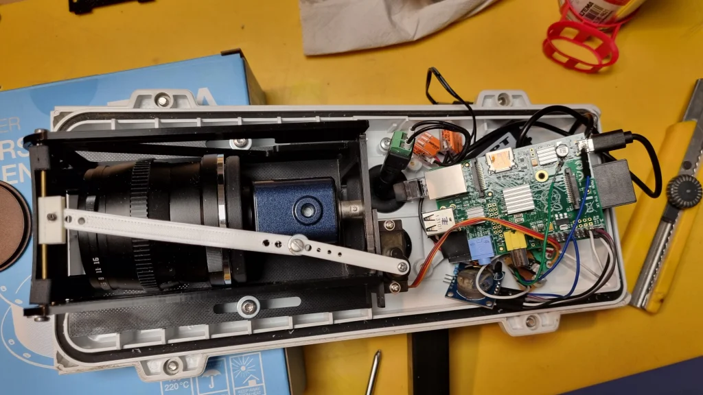
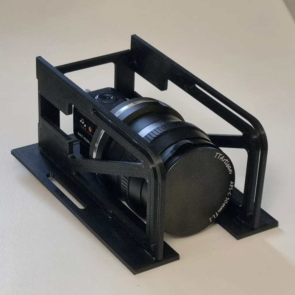
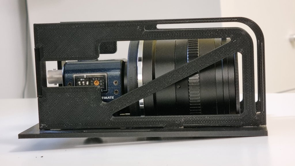
The software is Cees Bassa’s STVID and SATTOOLS. I have the camera in an IP68 camera housing with a servo driven sunshield in front of the lens. Separate mini PC has STVID doing the capture to a NAS storage in my network. A virtual machine has a STVID and SATTOOLS installed and I use it for processing the observations.

Scott Tilley – How did you feel when you first noticed the unidentified satellite in your data?

Tomi Simola – I was browsing the images that STVID had tagged as UNID. There was one set of images (20 or so) with an object with a rather short trail, meaning it was in a higher orbit. And while scrolling the images back and front I noticed the object was “accelerating”! The trail got longer (almost doubled) at the end of the set of images! Then I knew that this was something different!

My amateurish initial analysis for a circular orbit showed it in 56.5518 inclination, 6.6 revs/day. That inclination didn’t sound like Dr Marco Langbroek’s pre-launch prediction of 74 degrees. 6.6 revolutions per day was too much for a Molniya kind of orbit. I stated my doubts in an email to Seesat-L.

Scott Tilley – When did you know that you had found OTV7? How did that feel?

Tomi Simola – After Mike McCants email where he told me the UNID was OTV-7! I might have done a wild, but private “goal celebration”!

Scott Tilley – Can you tell us about your observing site and how it makes satellite observing unique? I.e. your northern latitude and how that affects satellite illumination.

Tomi Simola – My observing site is in my south facing backyard. But there is an area where I can set up my camera and point it over the neighbours roof, pointing low at the Northern sky. Area of the sky is busy with NOSS satellites which are very predictable and they are good targets to practice observations!

My latitude is 60 North, so some satellites are more visible earlier in the spring / later in the autumn, than for those in lower latitudes.

The site is very close to an international airport, but that has no great effect in my observations.

Scott Tilley – In this process of building an observing station and operating it what have you learned and what are your next steps?

Tomi Simola – I was not that much interested in visual satellite observing until two years ago, when I found the Watec camera for a very good price! Cees Bassa’s STVID was at that time getting rapid updates. Then I started to read tutorials from www.satobs.org.

I have done some RF observations with Bassa’s STRF (interest in this was sparked by Scott Tilley’s recovery of IMAGE in 2018), but the visual side was something different. SATTOOLS and STVID are very powerful software, but learning curve is…”steepish” – especially when one has no prior experience in visual satellite tracking!

Tutorials, articles and members of the Seesat-L have helped me to understand a bit better orbital dynamics and therefore I can pre-analyze my observations a bit better now. But there is so much more in orbital dynamics, visual tracking, that only way is forward! Interesting hobby that I never thought I’d get into!

More technical side, I have to improve the Wife-Acceptance-Factor of the camera setup. Also, a motorized mount would be nice in winter time!

Scott Tilley – Why do you look up and observe the sky to monitor satellites?

Tomi Simola – My interest in space flights and satellites was sparked when I was a small boy. I was living in a small village, far from the nearest city, with a stunning night sky! Moving stars in the sky were quickly explained as satellites.

The school library had lots of old books and my favourites were translated versions of “Die Mondlandung / Moon landing, 1969”, by Herbert J. Pichler and “Man and space, (Life science library), 1972” by Arthur C. Clarke. I have read these tens of times! I later acquired these books for my ever growing space library!

In my teens I received weather satellite pictures from NOAA and old Meteor satellites and kosmonauts talking with Moscow from MIR.

Satellites are fascinating! They are so close, just 200-300 km away, but getting there requires the smartest minds on the planet!

Spaceflights were for a long time only for superpowers and government backed institutions! They were rather rare occasions. Now, when technological advancements have brought satellites to the masses (you can almost literally buy your own satellite!), the “saturation” of the lower Earth orbit is getting more serious. I think satellite collisions are still rare, but astronomers using the whole electromagnetic spectrum (from DC to daylight and beyond) are getting frustrated with RF and visual noise in their data! Future space companies should have more responsibility to keep near space clean.

Amateur observers, not only for classified payloads, have an important task to bring these problems to the public and more importantly, to lawmakers! Good example is BLUEWALKER 3, which has a very large and visible antenna and dubious RF characteristics!

Conclusion

Once again amateur satellite observers with modest means and lots of patience find a classified object in space. We hope that sharing this story inspires others to look up and ensure the transparency in the use of space by all nations. 

Understand Doppler Analysis

We often post data online showing the results of a Doppler analysis. The concepts can be a bit intimidating to understand but with a little explanation it’s accessible to anyone.

Read more: Understand Doppler Analysis

What is the Doppler Effect?

When something emits electromagnetic radiation and is moving relative to an observer the observed wavelength of the emitting radiation will be different. Essentially when things are moving their movement effects how the waves of radiation arrive at the observer. If they are moving toward each other the wave crests successively arrive earlier thereby decreasing the wavelength observed. If the objects where moving apart then the opposite happens and the wavelength increases.

So how does this apply to observing satellites? Imagine you are at a very large train station that has an infinite number of tracks coming and going from the station in all directions. East, West, North, South and even up into the sky and down into the Earth. Further imagine you are listening to the whistles of all these trains passing through the station. Some are moving fast some slow all going in different directions. As almost everyone has experienced the pitch of the whistles note will change based on the change in velocity of the train as it passes you by. If you really pay attention you will notice the pitch of all the trains coming and going is different depending on their orientation to you, their speed and even if you decide to walk around the station and move yourself.

Using this knowledge one could use the Doppler effect to map out the train’s trajectories as they pass and determine which are which especially if they follow schedules and are on predefined routes. This is what we are doing to track satellites with the Doppler effect. Instead of whistles the satellites have radio transmitters. Instead of tracks they have orbits in which they are locked into by the force of gravity. These orbits are periodic and predictable. Therefore, if you know about how your moving and have observed data from the satellite’s radio transmitter you can compare this to a large number of guesses about the orbit it’s in and find matches that best fit the orbit. If you have a list of known satellites in known orbits you can compare that list to the data you collect to find the best match too.

All that is going on is systematically observing the change in frequency of the satellite’s radio emissions and then comparing that to a large number or educated guesses to find the best fitting guess to the data.

Understanding Doppler Analysis Plots

The following provides a brief walk through to orientate a reader on what Cees Bassa’s Satellite Tools Radio Frequency (STRF) displays as a result of a Doppler analysis of a signal. This should provide the reader with enough context to understand the display given our comments earlier.

The STRF Doppler Plot displays the raw Doppler data observed and the prediction of the Doppler from the current TLE (orbital model).

The Doppler plot noted above provides the raw Doppler frequency data (left y-axis) and the resulting range rate (line of sight velocity) on the right y-axis. The x-axis is time in Modified Julian Date (MJD).

Frequency is self evident as it’s the data we collect with our radio and antenna from the satellite. The range rate is a bit more obtuse. Range rate can also be better described as the line of sight velocity between two things. I.e. the resultant velocity at that time of perhaps two things moving with respect to each other. Doppler frequency tells us directly about this line of sight velocity and is what is actually used to compare the orbital models against.

Modified Julian Date (MJD) is a computationally friendly time system that allows for easy consecutive calculation of time based on a defined epoch (start date) of the system. MJD is used a lot in astronomy and astronautics.

Inside the plot the white lines (dots) are selected Doppler data. The grey line is the predicted Doppler curve when the object is below the observer’s horizon. The red line segments are when the object should be above the observer’s horizon.

The TLE (Two Line Element) block displays the current ‘template’ orbital elements being modelled.

The Two Line Element block displays the current ‘template’ orbital elements being modelled. If you want to learn more see my article on Basic Orbital Dynamics. The user can use template orbits, old orbits to update and also change the settings based on knowledge and intuition.

The Fitted Elements block allows the user to choose which elements should be fitted for the best fit to the data.

The fitted elements block allows the user to select which elements should be fitted for the best fit to the data. Careful selection of these given understanding of the orbital dynamics allows the user to find the best correct fit to a data set.

The Sky Track block provides a visualization of the satellites path through the observer’s sky during the times data is present.

The sky track block allows the user to visualize the satellite’s path through the observer’s sky during times data is present. This is helpful when comparing to other data sources like antenna position etc.

Analysis Results block provides the basic results of the current Doppler analysis.

The analysis results block provides the basic summary of the current Doppler analysis. Measurements is the total number of Doppler samples in the analysis. Frequency is the measured spacecraft emitted frequency once Doppler is accounted for. The rms is Root Mean Square error of the data compared to the model. TCA is Time of Closest Approach to the observing station performing the analysis. The name and COSPAR # for the observing station is next. The RED 8049 means that observing station 8049 data is present. If another station also contributed data their number and a different colour would be used to represent that.

To understand how good or bad an analysis is look at the rms number. The lower the better.

How Accurate is Doppler Analysis?

Accurate Doppler analysis relies on the observer recording very accurate frequency samples of the observed satellite signal. Therefore, using a very accurate clock for timing is required. In my case I use a GPS referenced oscillator to perform this function. This leads to the other source of error the spacecraft itself. Most spacecraft in Earth orbit and in Lunar orbit don’t usually have super stable radio oscillators. The reason is they don’t usually need this as the control stations will use other methods of determining the range and range rate to the spacecraft like two-way Doppler that uses a transponder on the spacecraft and therefore eliminates the spacecraft’s oscillator as a source of error. However, in our case we are limited to the one-way Doppler and must deal with the errors. If you want to learn more read NASA JPL’s Range and Doppler Tracking Observables.

STEREO-A Comes Home

STEREO-A is coming home in the summer of 2023 for the first time since it was launched 17 years ago and is providing amateur astronomers with a unique opportunity to do some citizen science. The spacecraft has inferior conjunction with Earth on August 17, 2023 and will be approximately 8.2 million kilometres distant then. While still far from Earth, STEREO-A will be unusually close to Earth and produce a unique opportunity to decode its deep space beacon and view stunning images of the Sun as it approaches solar maximum. In solving this riddle in the sky we present how we figured out how to decode STEREO-A’s images and present a suggestion of how to celebrate STEREO-A’s return to the vicinity of home.

Read more: STEREO-A Comes Home

Inferior Conjunction is not a Complex…

Inferior conjunction has nothing to do with a spacecraft having an unrealistic feeling of general inadequacy, rather it refers to its arriving at a position in it’s orbit where it lies between the Earth and the Sun. As you can see from the graphic below this is also the closest position STEREO-A can be to Earth in its given orbit.

Using this GMAT script here one can model the arrival of STEREO-A at inferior conjunction and and get a sense of the distances still involved. At closest approach STEREO-A will be a little more than 0.055 astronomical units (AU) from Earth. As we will see this has a profound impact of the radio signal from STEREO-A for listeners here on Earth.

Animation of STEREO-A approaching inferior conjunction with Earth. This is a rotating frame from the Earth’s perspective.

STEREO-A’s solar orbit with the Earth’s for comparison. Normally STEREO-A is quite far from Earth.

As one can note from the solar orbit of STEREO-A that it is quite similar to Earth’s orbit. But just a little faster so over a period of about 17 years STEREO-A will lap us and pass by for an inferior conjunction.

As noted above, this has a profound impact of the radio signal amplitude on Earth when STEREO-A is around inferior conjunction. The free space path loss (FSPL) of STEREO-A’s decreases with the square of the distance between Earth and the spacecraft. As can be seen on the plot below since STEREO-A was launched it has been on average very distant from Earth with a very large FSPL. But as inferior conjunction approaches the signal dramatically improves by about 30dB. The plots below show normalized signal strength levels relative to the peak signal level in the time period of the plot.

STEREO-A Range and Free Space Path Loss (FSPL) since launch.

Zooming in on the inferior conjunction event one can see the dramatic effect on the signal levels at Earth from the rapidly approaching STEREO-A spacecraft.

A zoomed in plot of STEREO-A’s range and FSPL around the August 17, 2023 inferior conjunction with Earth reveals the dramatic increase in the spacecraft’s signal.

Since about mid June 2023 the amateur radio station here with it’s small 66cm aperture dish antenna has been noticing a dramatic increase in signal levels and the emergence of data side-bands on the signal.

STEREO-A’s signal level in mid June 2023 on a small 66cm dish antenna. Notice the data side-bands are visible.

Once we’d figured out what was going on we found an obscure page on the STEREO Science Centre website that provides info on the conjunction and a tool to calculate STEREO-A’s position relative to the Earth, Moon and Earth-Sun L1 science missions.

Reception of STEREO-A Deep Space Beacon

You might be surprised to know that STEREO-A has a ‘deep space beacon’ that sends low rate data of the space environment and images of the Sun and surrounding area near constantly. It transmits +/- Doppler at 8443.58MHz.

The purpose of the beacon is to provide near real-time space weather forecasting ability. The real-time data from STEREO-A and other space weather monitoring missions at the Earth-Sun L1 point and in Earth orbit provide the world with a near constant flow of data on the space weather going on so we here on Earth can manage infrastructure that is sensitive to it such as power grids, satellite navigation and high frequency radio communication to name a few. This low rate data includes compressed images of some of the high resolution science data known as COR2, EUVI, HI1 and HI2 at an interval of few 10s of minutes depending on the payload. Other data it sends is numeric space weather data from the IMPACT, PLASTIC and S/WAVES payloads.

Presently there is a limited network of participating ground stations around the world that provide partial coverage to collect the real time forecast data from STEREO-A. The following stations are presently actively participating in STEREO-A space weather beacon reception and reporting the data to NASA for distribution.

  • APL: Johns Hopkins University Applied Physics Laboratory, Laurel, MD, USA
  • KSWC: Korean Space Weather Center, Jeju, South Korea
  • BOCH: AMSAT-DL/Bochum Observatory, Germany
  • KIEL: Amateur station DL0SHF, Kiel-Ronne, Germany
  • KOGA: National Institute of Information and Communications Technology: Koganei, Japan

One of the most interesting is the amateur station DL0SHF, a 7.5m dish antenna located in Germany that is run by amateurs and provides a Earth Moon Earth (EME) beacon service and also gathers data from STEREO-A. It is the smallest of the beacon monitoring stations that formally participates in data gathering for NASA.

The STEREO Space Weather Beacon Coverage as posted on NASA’s STEREO website. Marked on is the STEREO-A coverage provided by amateur station VE7TIL which presently is filling a gap in world wide coverage. Source: NASA STEREO Science Centre

The X-band station at VE7TIL used at present is right on the edge of working for STEREO-A deep space beacon reception a little over a month from its arrival at inferior conjunction. The dish antenna is a 66cm prime focus type and is mounted on a modified telescope mount to automatically track STEREO-A and other objects in space.

66cm prime focus dish antenna known as the Mighty Little Dish (MLD) is used for reception of STEREO-A deep space beacon signals as the spacecraft approaches inferior conjunction.

VE7TIL X-Band Dish Antenna Specifications:

66 cm at 50% illumination at 8.44 GHz is 32.3 dBi 

136K is 21.3 dBK. Hence G/T = +11 dB/K 

The overall system block diagram is provided below. This system has proved successful in hearing signals at Mars and in the vicinity of Mercury from BepiColombo as well as providing some great Earth images from LEO weather and science missions such as AQUA, TERRA, NOAA 21 etc.

X-Band system block diagram from the station at VE7TIL

Obtaining and Making Sense of STEREO-A’s Data

Back in 2022, Daniel Estévez, EA4GPZ published a blog post on Decoding the STEREO-A Space Weather Beacon where he used data obtained from the 13m dish at the Harbin Institute of Technology in China by amateur Wei Mingchuan BG2BHC to develop a demodulator and decoded the data into constituent components. Daniel’s work provided significant insight into STEREO-A’s low rate beacon signal structure and provided a means of plotting the S/WAVES experimental data. However, a vast majority of the data copied remained unknown and not decoded into the specific products being sent just the constituent data blocks containing the various sensors output’s. So much work was still to be done.

Alan Antoine, F4LAU, @Aang23, also added a demodulator to the SatDump tool kit which greatly simplified the demodulation of the signal as GNU Radio was not needed.

VE7TIL now had a signal from STEREO-A and a means to demodulate it but after some initial attempts no frames were decoded. Digging into SatDump a bit further the pipeline for the demodulator was found and the various parameters were tuned until near 100% demodulation and decoding of the STEREO-A signal resulted. Due to the low SNR tuning the PLLs very tightly resulted in the most significant improvement in the performance of the system. The updated parameters used can be found here. As SNR improves these tight values don’t really improve performance much, but at low SNR they helped dramatically.

 "pm_demod": {
                    "symbolrate": 3800,
                    "resample_after_pll": true,
                    "agc_rate": 0.0005,
                    "pll_bw": 0.0025,
                    "pll_max_offset": 3.14,
                    "rrc_alpha": 0.2,
                    "rrc_taps": 31,
                    "costas_bw": 0.0001,
                    "clock_omega_relative_limit": 0.005
                }
            },
            "frames": {
                "ccsds_turbo_r6_k8920_decoder": {
                    "turbo_iters": 20

So how can an amateur station with such a small antenna have a hope of demodulation of spacecraft over 15 million kilometres away? The secret is the Turbo coding used by the spacecraft to encode it’s signal. As Daniel noted in his analysis STEREO-A uses the most robust method available from the standard.

The symbol rate is 3.8 kbaud. The FEC is CCSDS Turbo coding with r=1/6 and 8920 informations bits. From the different FECs described in the TM Synchronization and Channel Coding Blue Book, this is the one that gives the best Eb/N0 performance.

Daniel Estévez

In the image below one can see just how marginal the demodulation and decoding of the STEREO-A signal is and also appreciate the incredible performance of the Turbo code used to make this possible as it approached the Shannon limit.

The SatDump demodulator and decoder in action on STEREO-A’s signal as copied by VE7TIL.

As noted above the data is sent at a very low rate, so to gather a MB of data takes hours. But after patient waiting one is rewarded with a data file full of STEREO-A data and many compressed images.

A byte raster of STEREO-A raw binary data.

Daniel had largely made sense of the major structures in the data and gave clues as to where to look to build on finding and extracting image and further numeric science and telemetry data from the data.

This is where Alan did some detective work on the STEREO Science Centre website and found some tidbits of information and code that made the process of finding the images and then decompressing them to allow us to view the raw images being sent from STEREO-A via its low rate deep space beacon.

Alan found the document that describes the STEREO/SECCHI Level-0 to Level-0.5 FITS Pipeline CMAD on the STEREO website and two C files, rdSc.c and hdr.c in a directory on the STEREO site /instruments/software/secchi/utils/rdSh. These documents provide considerable insight into how the data from the spacecraft is processed on the ground to be used for generating images. The proceeding document provided details on some formats that were used to figure out the packet format and know how to extract the header, data, and trailer block and allowed Alan with a bit of reverse engineering to gather together the first image files by extracting the header, data, and trailer blocks from the raw data files.

The next step unique to this mission was to decompress the highly compressed deep space beacon images. Alan found a Linux binary on the STEREO site that did the job. Called ‘idecomp.linux’ it decompressed the data so an image could be extracted and viewed. Unfortunately, the source code hasn’t been found yet as NASA doesn’t have a copy, we asked! We’re exploring other avenues to obtain the source code for integration into SatDump to make the extraction of images from STEREO-A not platform dependant.

You need to download the idecomp.linux file and change the Stereo.json file in the SatDump pipelines folder to direct your version of SatDump to the local path of the executable. Ensure you have the latest build of SatDump before setting this up.

"products": {
                "stereo_instruments": {
                    "icer_path": "./icer_decomp_linux"

Alan’s SatDump code found in the GITHUB SatDump repository tells all the gory details of how the images are extracted and decompressed for those seeking those details.

A summary of the process of extracting STEREO-A data and images is as follows:

  1. Demodulate: Convert the modulated signal back to its original form.
  2. Correlator: Use correlation techniques to detect and synchronize the received signal.
  3. De-randomize: The bit stream is de-randomized. It is randomized to ensure synchronization is possible and a clean modulation
  4. Turbo Decoder: Employ turbo decoding techniques to recover the original data.
  5. VCID Selection: Choose the appropriate Virtual Channel ID (VCID) to process.
  6. Extract CCSDS Packets: Extract CCSDS Packets from the data stream and filter by APID.
  7. Recompose File Blocks: Reassemble the packets into their respective file blocks.
  8. Dump Payload Part: Isolate the payload part of each file block.
  9. Decompress: If the payload is compressed, decompress it to obtain the original data.
  10. Image: Process the decompressed data as an image.

Further a review of the actual FITS images found in the beacon data files provided a further clue as to how to identify the APID, telescope and unique image information. The raw binary data from the spacecraft also includes ASCII filenames found to correlate with the source filenames located in the FITS headers of the images found on NASA’s STEREO website. Alan’s work revealed that the SECCHI images raw off the spacecraft were not the images seen on the SECCHI beacon summary site and this caused us some initial confusion about what the actual APIDs were for each type of image until we unlocked the riddle of the ASCII filenames.

Spacecraft binary stream with ASCII image filename highlighted.
Here the FITS image file header corresponding to the data heard from STEREO-A by VE7TIL is found to contain the image filename in the FILEORIG field.

Further research on the STEREO website lead to finding the filename convention for images sent by STEREO-A and B in a document called SECCHI FITS Header Keyword Definition, page 12. So the filename is a very powerful tool to identify all this info in a compact way. Based on our experience thus far this is the only ASCII data sent by STEREO-A.

EXAMPLE:

Filename format is YMMDDaaaa.APT

Where,
Y = Year
MM = Month
DD = Day
aaaa = image counter and sequence number
AP  = APID
T = Telescope used

Decoding filename N63004MD.743

Given,
N =  'N' in base 36 is equal to 23 in decimal, thus the year from 2000
6 = is the month of June, note this is also in base 36
30 = is the day of the month
04FM = is the image counter & sequence number in base 36
. = extension point
74 = APID 1140, given that the APID in hex minus 0x400, i.e. 0x474 - 0x400 = 0x74

Where, APID 1137 (0x471), 1138 (0x472), 1139 (0x473) and 1140 (0x474)

3 = The telescope is EUVI

Where, 1=COR2, 2=COR1, 3=EUVI, 4=HI2 and 5=HI1, for STEREO-B add 5.

Further research turned up some processing code on the NASA STEREO site that revealed other image filename extensions and their relationships to the naming conventions used in the data repository on the NASA site called getscifileinfo.pro.

Excerpt from getscifileinfo.pro that relates filenames, APID and telescopes together.

With the knowledge extracted from the spacecraft data, and the NASA STEREO website a complete understanding of the presently observed APIDs was obtained and this was cross referenced with data received from STEREO-A and that recorded on the NASA website as a double check. The table below provides a convenient summary.

The table provides a summary of known APID use on STEREO-A. Based on the information found the 1136 should be in use for the COR1 telescope but has not been observed in the data thus far.

Behaviour of the STEREO-A Beacon

STEREO-A has largely two modes of normal operation. High rate data while in lock with a ground station and low rate data when not in lock and sending deep space beacon data including the compressed images used for space weather forecasting.

Understanding the beacon’s behaviour and knowing how to plan observing sessions to gather the deep space beacon data is important. The following spectra show the unlocking/locking behaviour when STEREO-A ends and starts DSN communications. You can plan your observing sessions around the DSN sessions by referring to the STEREO DSN Schedule Summary posted on the STEREO-A website.

DSN Now doesn’t show all the activity as other ground stations from ESA and NASA ones not on the live website are used and we’ve noted a few times where the STEREO-A schedule shows activity which we can see happening on the air but the DSN NOW site shows no activity for the respective deep space station antenna. So the STEREO-A website schedule appears the golden source of scheduling info.

Overview of STEREO-A unlocking from DSS65 in Madrid, sending low rate deep space beacon data and then locking with DSS14 in Goldstone
STEREO-A ends high rate data (carrier only visible) begins low rate data and unlocks from DSS65 in Madrid.
Just before locking to DSS14 in Goldstone STEREO-A for some reason toggles lower in frequency and pops back up. This caused the decoder to briefly unlock.
STEREO-A locks to DSS14 in Goldstone. Note, it has ended low rate data before entering into the locking sequence.

The data download speed is very low and to gather images long data gathering runs are needed. To gather enough for animations entire passes should be recorded.

Doppler rates will be dramatically changing as STEREO-A approaches and passes inferior conjunction. The plots below will provide an overview since launch and a zoomed in analysis of the Doppler resulting around the inferior conjunction.

STEREO-A Range Rate and Doppler since launch and through the Inferior Conjunction.
STEREO-A Range Rate and Doppler data zoomed in around the time of the Inferior Conjunction on 2023-08-17.

The best strategy for demodulation/decoding the data is to setup and make a long recording of STEREO-A’s low rate data when the spacecraft is not in a high rate data session with a ground station. Record lots of data (more than an hour) and then run the SatDump decoder and allow the signal to lock and write the .cadu file and then process the images. The lower the SNR you have the longer the decoder needs to lock onto the signal and start producing data. Since STEREO-A sends it’s data at such a low rate you need to record for long periods of time to get many images.

The Glorious Images!

STEREO-A colour composite of the EUVI 195 and 304 images showing the peak of an X-Flare at 2023-07-02T23:20 UTC
STEREO-A EUVI 304 animation revealing a huge naked eye sunspot that X-flares!
STEREO-A EUVI 195 animation also clearly showing the X-flare saturating the imager.
STEREO-A COR2 animation revealing Mercury passing behind the Sun at superior conjunction with the Earth.
STEREO-A HI1 animation. Stars and Solar Corona.

A complete repository of all the images used to make these animations and the raw data recovered by STEREO-A during this process can be found here.

Inferior Conjunction Citizen Science Opportunity

STEREO-A will be quite close to Earth for some months to come and some amateurs with larger dish antennas have been able to decode STEREO-A for about a year now. This proximity provides a unique opportunity for amateur observation of the STEREO-A signal and the recovery of data from the low rate beacon that may fill some data gaps in the present system. Being that it’s near solar maximum gathering of the this data in near real-time with limited gaps may be of value to space weather forecasters as amateurs can fill in gaps in the existing low rate beacon receiving network.

There are plans to allow for the real time data from a running SatDump STEREO-A receiving system to be posted to the Internet and allow NASA or any other interested party access to the raw data so it can be processed and used as they see fit. This would allow the growing community of deep space network radio observers to contribute to science and the forecasting of space weather events during a time of higher than usual solar activity and allow all involved to learn more about the Sun and the resulting space weather it creates.

This is a unique way the world can celebrate the first inferior conjunction of the 17 year old STEREO-A mission!

Welcome home STEREO-A may you have another inferior conjunction in you.

Acknowledgements

Alan Antoine, F4LAU – The driving force behind the open source SatDump software package for the decoding of satellite imagery. He provided the decoder and the expertise to extract the images from the STEREO-A data stream while teaching this old dog some new tricks!

Daniel Estévez, EA4GPZ – Rigorously documents each deep space mission to learn about it signal’s characteristics and reports many educational details on his highly useful blog to the amateur radio community. Daniel’s work laid the groundwork for us to carry on the study of STEREO-A’s signal.

USA SATCOM – Joe provided data from his impressive 2.3m X-band system and filled in gaps at times to help improve the rigour of our data analysis. USA SATCOM offers a range of highly reliable software in Windows for tracking, decoding and presenting space based imagery.

Paul Marsh (UHF SATCOM) and Jean-Luc Milette for reporting the ever increasing STEREO-A signal and prompting me to wonder what was going on.

Dr. Cees Bassa – It goes without saying that Cees’ work on STRF (SatTools RF) makes for easy and accurate work on any form of Doppler analysis project. See his GITHUB site for code and details. Thank-you Cees!

NASA STEREO Science Centre – A shinning example of open space science to be modelled by other missions and agencies. Many thanks to the team for timely responses to questions and their proactive open behaviour in sharing mission data and operational details.

A Global Chinese Space Based Short Message System

Recent media reports indicate the US has developed a way to track the recent Chinese airships passing over North America. Here, a hypothesis is offered on how this may work and how observers can contribute.

In July of 2022, the Chinese commercial JILIN Earth imaging constellation of satellites was found to be emitting strange short burst data signals on spectrum reserved for the mobile-satellite (Earth-to-Space and visa-versa) radio service. This observation while curious at first caused the author to reconsider the meaning of that observation after the recent arrival of a large Chinese airship over North America and how it may communicate with its handlers as a bit more research revealed a clear connection to the Chinese BeiDou satellite navigation system and the emissions from JILIN.

Continue reading “A Global Chinese Space Based Short Message System”

Mysterious ‘Pips’ from the Chinese JILIN Constellation

Why is an imaging satellite constellation acting like a mobile-satellite communications system?

China’s first self-developed commercial remote sensing satellite system known as JILIN is sending strange wideband data pips in a quiet piece of spectrum on L-band. The JILIN system is operated by Chang Guang Satellite Technology Company in Beijing. No public references have been found by the author about what these emissions from the satellites purpose is.

Continue reading “Mysterious ‘Pips’ from the Chinese JILIN Constellation”

You can call me Dmitry Meyer…

History Repeats Itself

Russia operates a constellation of satellites in high Earth orbit called Meridian (меридиан). These satellites perform a critical communications purpose for Russia as much of its land mass is not well served by geostationary satellites. Therefore, you would think this constellation would be held to the highest operational level. Well it’s not as radio amateurs have observed. This fact could raise questions about Russia’s ability and preparedness to act on their recent veiled threats of nuclear war.

Continue reading “You can call me Dmitry Meyer…”

Chang’e 5 Returns to the Moon

Chang’e 5 has quietly departed from the Sun-Earth L1 point to enter a distant retrograde orbit (DRO) of the Moon, a first.

Pre-empting NASA’s planned 1st use of the orbit during Exploration Mission 1 later this year.

Silence from China.

Off Station

In mid August 2021, the Chang’e 5 service module without any notice was noted to not be on station near the Sun-Earth L1 point where it had been since mid-March 2021. Observers were quick to reacquire the spacecraft’s X-band beacon and it was not long before it was clear from the data that Chang’e 5 was headed back to the Earth-Moon system where it would ultimately enter a Distant Retrograde Orbit (DRO) of the Moon.

Continue reading “Chang’e 5 Returns to the Moon”

Understanding LES-5’s Power System Status

It’s be a quarter of a year since LES-5 was recovered and we began decoding telemetry.  The spacecraft sends 128 words (8 bit bytes) every 10.24 seconds which is called a format.  That format is comprised of four frames of 32 words.  Of the 128 words eight are used for syncing and 24 used for parity checking.  This leaves 96 that contain telemetry data.  Until now we only fully understand eight of the words used for the Radio Frequency Interference (RFI) experiment, leaving 88 words with unknown meaning.  What follows is how we determined the meaning of four more words that reveal the health of LES-5’s solar power system and the present rotational period of the spacecraft.

Continue reading “Understanding LES-5’s Power System Status”

Recovering Iran’s NOUR 01 ‘Military Satellite’

Iran’s new military satellite, NOUR 01, most interesting fact may not be that it resembles a college engineering experiment but rather that it may have a connection to a Mexican military payload launched quietly from New Zealand last year.

It’s also with great pleasure that I can share Scott Chapman, K4KDR’s story of how he found Iran’s NOUR 01 [45529, 2020-024A] radio emissions and confirmed it was alive and well in orbit and noted a twist to the story in a brief interview we had.

Continue reading “Recovering Iran’s NOUR 01 ‘Military Satellite’”

A Brief Look at LES-5’s Telemetry Format

It’s not exactly every day that you get the chance to work with any data, let alone telemetry data from a 50-year-old satellite. However, thanks to Scott’s observations of LES-5 and subsequent investigation into its telemetry beacon, the opportunity arose. Based partly on the work of others, as well as what I’ve managed to glean from the technical documentation that has been gathered, I’d like to explain my process for processing data from LES-5.

Continue reading “A Brief Look at LES-5’s Telemetry Format”